Data analysis (Module 2, p. 1/2)
This part of the text provides brief summary of our key findings on Module 2 followed by a detailed exhibition of our empirical analysis. We first present some of the most important data characteristics followed by a description of the data preparation process. On the basis of the performed preliminary analysis we chose random forest as our core modelling approach. At the same time, the stage of preliminary analysis supports the process of feature engineering. The latter is presented in greater detail as it forms an important contribution both to the topic of Sofia air pollution modelling as well as to the general strand in literature engaged with air pollution predictive models. Next, we present results of model estimation and highlight which variables are the strongest predictors. Out-of-sample prediction accuracy is reported at the end of the section.
Summary of key findings
- We build a predictive model via the random forest approach.
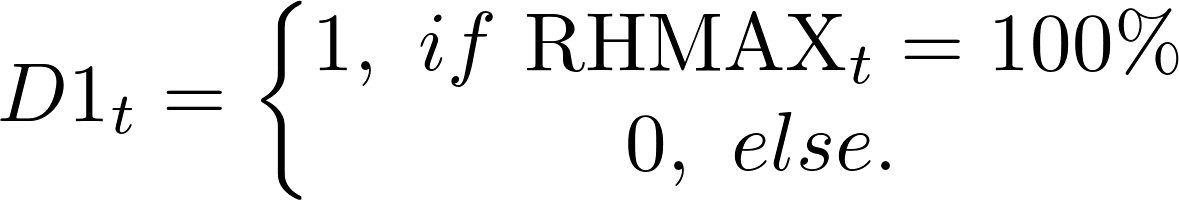
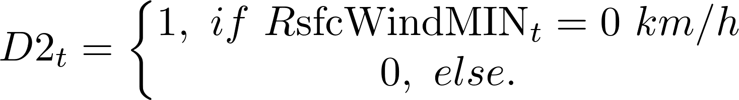
- Whenever the level of PM10 is above** 50 µg/m3 we note that the maximum relative humidity is 100%, also the minimum wind speed is 0 km/h and the average precipitation amount is 0 mm. Therefore, **introducing dummy variables allowing for this fact would help in modelling the extreme air pollution levels.
- Weak to moderate correlation is observed between the level of PM10 concentration and the available weather indicators. The highest values are slightly below 0.45 in absolute terms and they correspond to the correlation between PM10 and pressure indicators as well as to PM10 and temperature indicators. Therefore, introduction of additional features is necessary.
- Strong linear dependence is observed between groups of weather indicators (e.g. all indicators corresponding to temperature and dew point temperature are severely correlated). Therefore, feature selection is required.
- The most important variable in predicting the air pollution in Sofia is the Ratio of the previous day concentration of PM10 and the cross-product of current and previous day wind speed.
- Previous day concentration of PM10 and the cross-product of current and previous day wind speed are also essential predictors.
- Season (month), temperature, humidity and pressure are of secondary importance in explaining the variation in the level of air pollution.
- The latter findings suggest that other factors (such as road traffic intensity, etc.) that are absorbed to certain extent in the previous day concentration of PM10 might cause the huge impact captured by the synthetic variables R,CP,lagP1. Therefore, enriching the feature space with additional information might be helpful in identifying the drivers behind their high values.
- Delivered accuracy measures suggest next-day forecasts generated by our predictive models outperform considerably the naïve forecast. Additionally, achieved accuracy is comparable with that reported in similar studies (see for example Table 3 at p. 596 of (Kurt, et al., 2008)). At the same time, our approach preserves interpretability of results and we consider this an important contribution of our research.
Empirical Analysis
This part of the text provides detailed information on the performed empirical analysis related to Module 2 of our research. The flowchart at presents the core stages of our analysis.
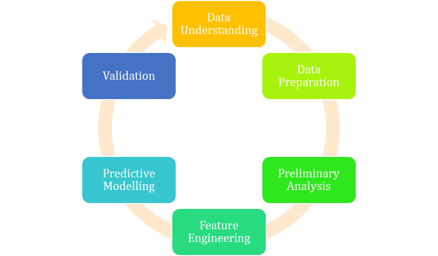 Figure 8: Empirical analysis of Module 2: Workflow.
Data Description (Understanding)
Module 2 is based on time series data of PM10 concentration measurements at five official stations in Sofia as published by the European Environment Agency. The raw data is hourly sampled. Table 1 summarizes more important data characteristics.
Table 1: Descriptive statistics of hourly PM10 concentration measurements at the official stations in Sofia.
| Station code | 9421 | 9572 | 9616 | 9642 | 60881 |
|---|---|---|---|---|---|
| Start date and time | 2017-12-02 18:00:00 | 2017-12-02 18:00:00 | 2017-12-02 18:00:00 | 2017-12-02 18:00:00 | 2018-01-01 02:00:00 |
| End date and time | 2018-09-14 23:00:00 | 2018-09-15 00:00:00 | 2018-09-15 00:00:00 | 2018-09-15 00:00:00 | 2018-09-14 20:00:00 |
| Number of obs. | 6869 | 6870 | 6870 | 6870 | 6162 |
| Number of NAs | 316 | 185 | 834 | 254 | 165 |
| Mean | 18.98 | 34.07 | 35.63 | 33.49 | 30.32 |
| Median | 13.39 | 23.10 | 25.02 | 24.07 | 22.78 |
| Min | 0.09 | 2.12 | 4.03 | 0.30 | 5.45 |
| Max | 298.55 | 689.65 | 479.30 | 419.12 | 483.37 |
| 1st Quartile | 9.08 | 15.44 | 17.88 | 16.35 | 16.41 |
| 3rd Quartile | 20.11 | 34.79 | 36.97 | 34.92 | 31.68 |
As might be seen hourly measurements has extreme maximum values and asymmetric (left-skewed) frequency distributions. Also, one of the stations (coded as 9642) is characterized by higher number of missing observations amounting to approximately 12% of the entire sample. The latter findings suggest that:
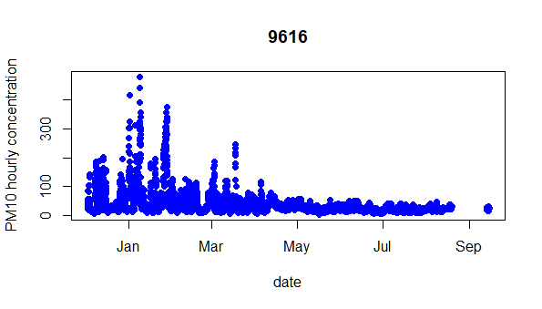 Figure 9: PM10 hourly concentration measured at station 9616.
- Data interpolation should be introduced. As might the seen from Figure 9 , a long period is missing for station 9616. Therefore, we should apply conservative interpolation technique.
- Averaging observations on daily basis would reduce noise and asymmetric distributional properties. Furthermore, the level of PM10 concentration is subject to regulations on average 24-hours basis.
The second source of data consists of meteorological information published by Sofia Airport Weather Station. The observations are with daily sampling rate. Table 2 presents summary of available variables.
Table 2: Meteorological indicators published by Sofia Airport Weather Station: Summary and notation.
| Variable name | Variable Label | Units of measurement | Number of NAs |
|---|---|---|---|
| TASMAX | Daily maximum temperature | degrees C | 4 |
| TASMIN | Daily minimum temperature | degrees C | 4 |
| TASAVG | Daily average temperature | degrees C | 4 |
| DPMAX | Daily maximum dew point temperature | degrees C | 4 |
| DPMIN | Daily minimum dew point temperature | degrees C | 4 |
| DPAVG | Daily average dew point temperature | degrees C | 4 |
| RHMAX | Daily maximum relative humidity | Percent | 4 |
| RHMIN | Daily minimum relative humidity | Percent | 4 |
| RHAVG | Daily average relative humidity | Percent | 4 |
| sfcWindMAX | Daily maximum wind speed | km/h | 4 |
| SfcWindMIN | Daily minimum wind speed | km/h | 4 |
| sfcWindAVG | Daily average wind speed | km/h | 4 |
| PSLMAX | Daily maximum surface pressure | Hpa | 4 |
| PSLMIN | Daily minimum surface pressure | Hpa | 4 |
| PSLAVG | Daily average surface pressure | Hpa | 4 |
| PRCPMAX | Daily maximum precipitation amount | Mm | 288 |
| PRCPMIN | Daily minimum precipitation amount | Mm | 288 |
| PRCPAVG | Daily average precipitation amount | Mm | 4 |
| VISIB | Daily average visibility | Km | 49 |
We might note that daily maximum and minimum precipitation amount variables consist of missing values only. Also, daily average visibility has altogether 49 missing observations. After careful inspection we find that missing values correspond to the last 49 days in our sample.
Data Preparation
As explained in section 4.2.1 we would first interpolate missing values. Linear interpolation is applied as more flexible opportunities such as spline interpolation are not well-suited in case of long consecutive periods of missing data. As a next step of our analysis hourly PM10 measurements by stations are aggregated on daily basis through averaging in time. The more important descriptive statistics of the transformed dataset are summarized in Table 3.
Table 3: Descriptive statistics of daily PM10 concentration measurements at the official stations in Sofia
| Station code | 9421 | 9572 | 9616 | 9642 | 60881 |
|---|---|---|---|---|---|
| Start date and time | 2017-12-02 | 2017-12-02 | 2017-12-02 | 2017-12-02 | 2018-01-01 |
| End date and time | 2018-09-14 | 2018-09-15 | 2018-09-15 | 2018-09-15 | 2018-09-14 |
| Number of obs. | 287 | 288 | 288 | 288 | 257 |
| Number of NAs | 0 | 0 | 0 | 0 | 0 |
| Mean | 19.55 | 35.00 | 35.51 | 34.29 | 30.63 |
| Median | 14.60 | 25.58 | 27.60 | 26.05 | 23.73 |
| Min | 4.09 | 7.68 | 8.16 | 9.22 | 9.44 |
| Max | 150.04 | 267.06 | 221.73 | 184.66 | 265.28 |
| 1st Quartile | 11.19 | 18.97 | 20.52 | 20.03 | 19.10 |
| 3rd Quartile | 19.55 | 33.42 | 35.95 | 34.21 | 31.09 |
| Number of days above 50 µg/m3 | 15 | 35 | 45 | 30 | 23 |
Regarding the meteorological dataset, the following preparation steps are performed. First of all, we remove daily maximum and minimum precipitation amount variables. We also remove the visibility variable, as filling the long period of missing values might impact results. Finally, missing observations for the rest of the meteorological variables are handles via linear interpolation.
Preliminary (Exploratory) Analysis
The very first step of our preliminary analysis comes down to test the time series of PM10 measurements at the analyzed official stations for stationarity. Figure 10 presents the autocorrelation function (ACF) for each of the analyzed times series on PM10 average daily concentration. We might note that all of the time series are characterized by fast decaying ACF so we can conclude on stationarity. This finding is supported by the augmented Dickey-Fuller test results, reported in Table 4.
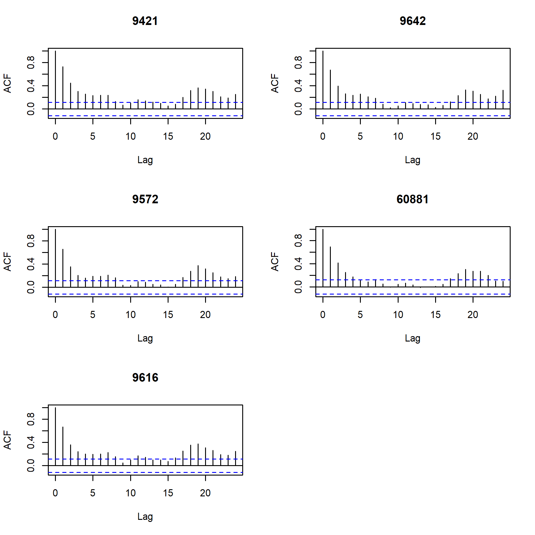 Figure 10: Autocorrelation function of PM10 concentration. Each panel corresponds to one of the official stations.
Table 4: Augmented Dickey-Fuller test results.
| 9421 | 9572 | 9616 | 9642 | 60881 | |
|---|---|---|---|---|---|
| ADF statistics | -4.79708 | -4.822 | -4.933 | -5.16014 | -4.79295 |
| p-value | 0.01 | 0.01 | 0.01 | 0.01 | 0.01 |
The next step of our preliminary analysis investigates the dependence between the concentration of PM10 and the weather indicators. In text that follows, we report results only for one of the stations (this is station 9421) because similar dependencies are observed for rest of the stations (find rest of the results in section Appendix M2.). Figure 11 provides pairwise scatterplots where the x-axis represents particular weather indicator, while the y-axis corresponds to the level of PM10 concentration. Figure 12 presents the correlation matrix in absolute terms via color code, where hotter colors correspond to stronger linear dependence.
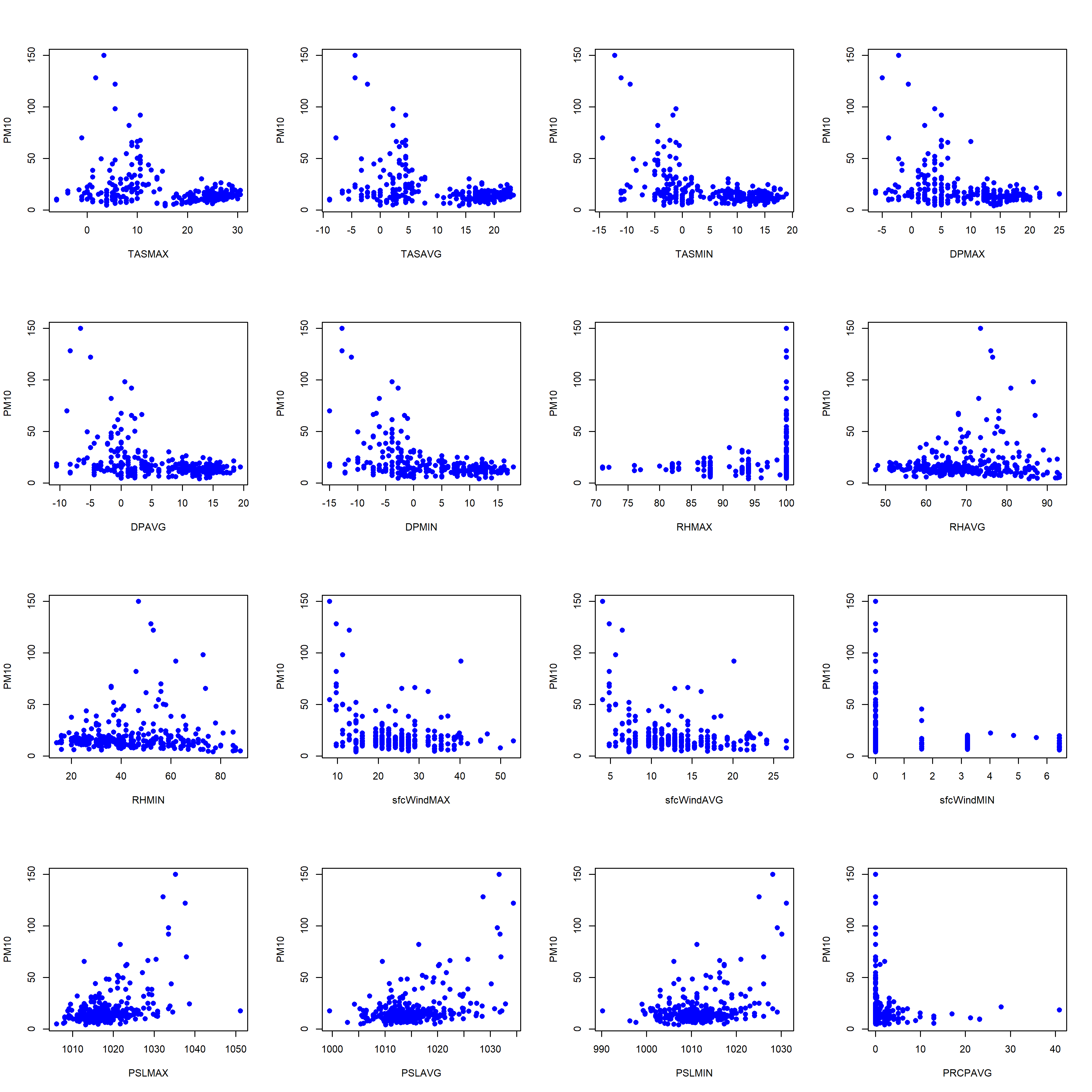 Figure 11: Pairwise scatterplots for station 9421. The x-axis represents particular weather indicator, while the y-axis corresponds to the level of PM10 concentration.
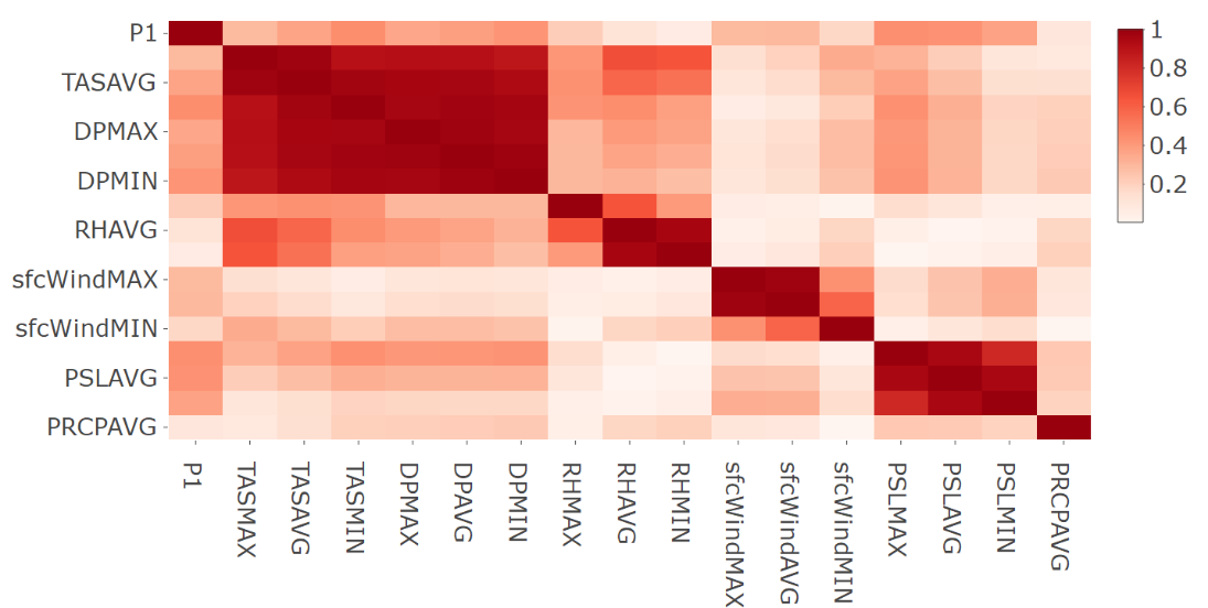 Figure 12: Correlation matrix in absolute terms for station 9421.
On the basis of Figure 11 and Figure 12 we might outline the following important data characteristics.
- Techniques based on feature space partitioning , i.e. tree-based algorithms are preferred to linear models. Therefore, we build a predictive model via the random forest approach.
- Whenever the level of PM10 is above** 50 µg/m3 we note that the maximum relative humidity is 100%, also the minimum wind speed is 0 km/h and the average precipitation amount is 0 mm. Therefore, **introducing dummy variables allowing for this fact would help in modelling the extreme air pollution levels.
- Weak to moderate correlation is observed between the level of PM10 concentration and the available weather indicators. The highest values are slightly below 0.45 in absolute terms and they correspond to the correlation between PM10 and pressure indicators as well as to PM10 and temperature indicators. Therefore, introduction of additional features is necessary.
- Strong linear dependence is observed between groups of weather indicators (e.g. all indicators corresponding to temperature and dew point temperature are severely correlated). Therefore, feature selection is required.
Feature Engineering
Based on the findings documented in section Preliminary Analysis we define the feature matrix that is used for the predictive model building.
We first make feature selection on the basis of the correlation analysis as well as taking into account results documented in the literature. In particular, the research of (Kurt, et al., 2008) uses weather indicators that are similar to those available from the Sofia Airport Weather Station. The authors suggest the following indicators as input in their model: weather condition, day and night temperature, humidity, pressure, wind speed and wind direction, day of the week. Therefore, minimum and maximum temperature, average humidity, and average pressure are initially selected. Instead of taking directly the observations on wind speed, we use them to construct an additional feature as explained in the next paragraph.
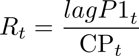
As explained in the previous section, we consider that feature engineering plays crucial role in the construction of accurate predictive air pollution models. The reviewed literature suggests that lagged values of PM10 concentration are strong predictors. Consequently, we refer to the partial ACF (PACF) presented at Figure 13 in order to determine the number of relevant lags. The figure suggests that only the first lag impacts significantly the level of PM10 concentration therefore we include it in the feature matrix as lagP1. The lag effect is further considered with regard to the fact that the city of Sofia is located in a hollow , i.e. in case of high concentration of PM10 in the previous day as well as no or weak wind both during the previous and during the current day, we might expect high concentration of PM10 for the current day. This motivates introduction of two additional features:


Finally, we introduce the day of the week and the month as predictors. The reader might find summary of features that are used in the next stage of the empirical analysis in Table 5.
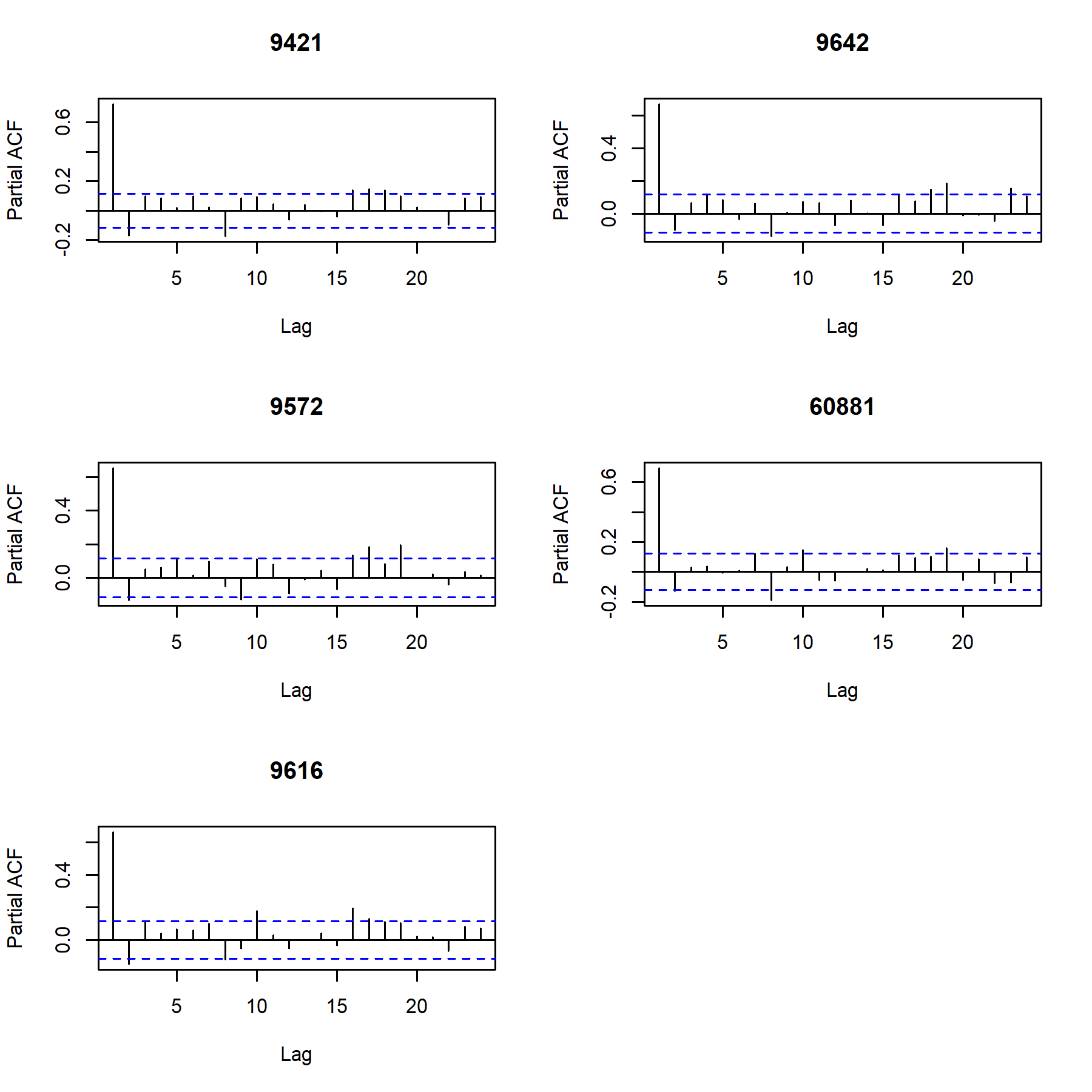 Figure 13: Partial autocorrelation function of PM10 concentration. Each panel corresponds to one of the official stations.
Table 5: List of features used for prediction purposes.
| Variable name | Variable Label |
|---|---|
| TASMAX | Daily maximum temperature |
| TASMIN | Daily minimum temperature |
| RHAVG | Daily average relative humidity |
| PSLAVG | Daily average surface pressure |
| lagP1 | Previous day concentration of PM10 |
| CP | Cross-product of current and previous day wind speed |
| R | Ratio of the Previous day concentration of PM10 and the cross-product |
| D1 | Dummy variable reflecting the case of 100% maximum humidity |
| D2 | Dummy variable reflecting the case of 0 km/h minimum wind speed |
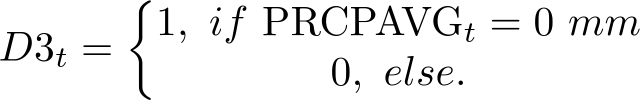
| D3 | Dummy variable reflecting the case of 0 mm average precipitation amount |
| D | D1*D2*D3 |
| day | Day of the week |
| month | Month of the year |
Figure 14 presents the correlation matrix in absolute terms for the response and selected features variables for station 9421. Similar results for the rest of the stations are reported in the Appendix at the end of section 4.
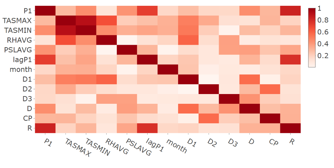 Figure 14: Correlation matrix in absolute terms for the response and selected features variables for station 9421
Predictive Modelling
In this section we use the random forest approach so as to deliver nonlinear prediction model for each of the official stations. For this purpose we define Algorithm 1.
- Split data on random basis into two subsets (train and test) of equal length.
- Fit random forest equation with 500 trees.
- Record equation and other control information.
- Perform 1 day ahead forecast over the test set.
- Calculate out-of-sample RMSE and MAE.
- Repeat steps 1 to 5 until 100 iterations are reached. Average results on variable importance, RMSE, MAE. Algorithm 1: Algorithm for iterative application of the random forest approach to moderate sample size.
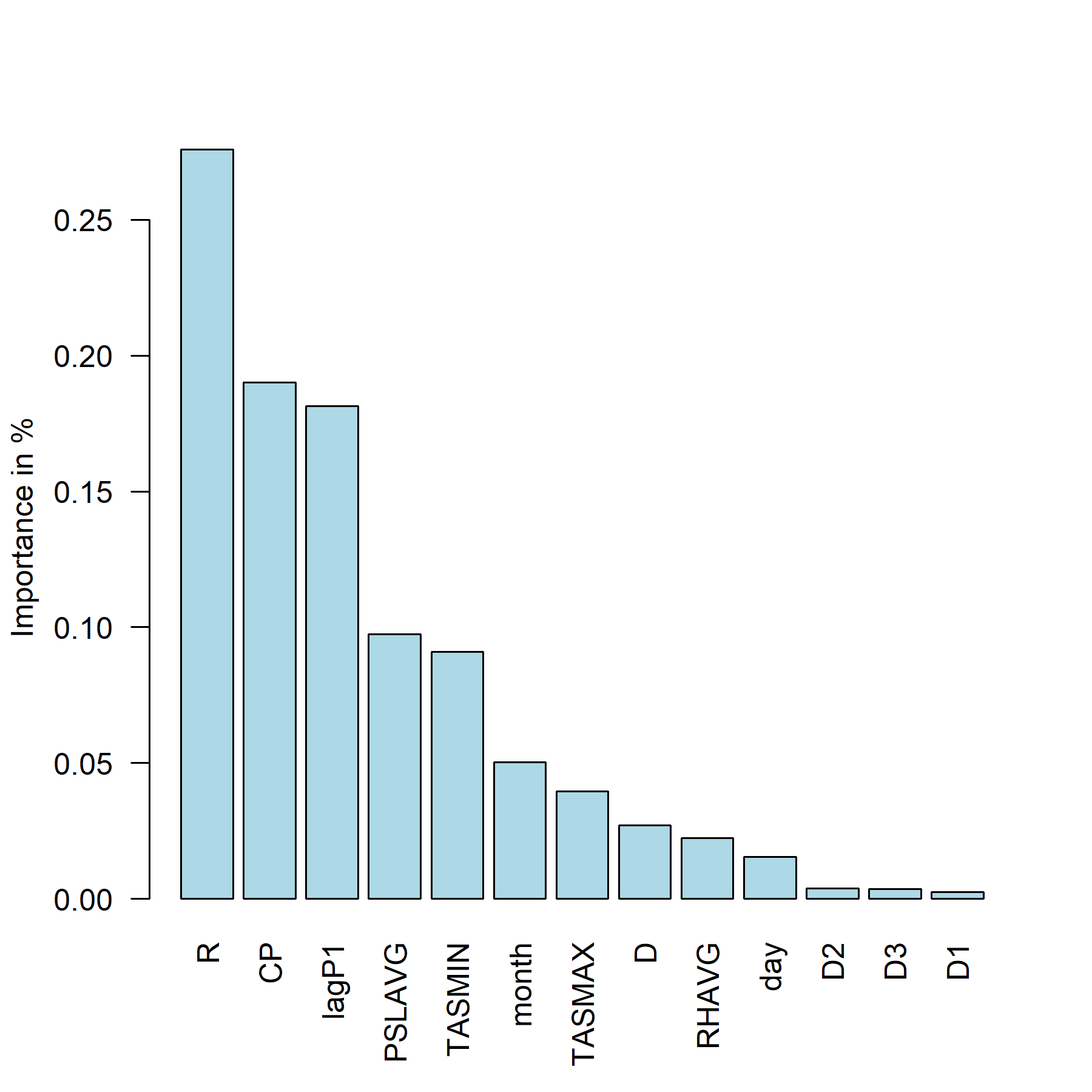
Figure 15: Summary of feature importance expressed as percentage of the cumulative decrease in the optimized loss function. Station 9421.
It is worth noting that the algorithm assures robustness of results to the random sampling process. Thus we deliver predictive equations and out-of-sample forecasts for all of the official stations. Estimation results are similar therefore we report variable importance diagram for station 9421 at Figure 15 , while results for rest of stations might be found in the Appendix at the end of Section 4. The following conclusions might be drawn:
- The most important variable in predicting the air pollution in Sofia is the Ratio of the previous day concentration of PM10 and the cross-product of current and previous day wind speed.
- Previous day concentration of PM10 and the cross-product of current and previous day wind speed are also essential predictors.
- Season (month), temperature, humidity and pressure are of secondary importance in explaining the variation in the level of air pollution.
- The latter findings suggest that other factors (such as road traffic intensity, etc.) that are absorbed to certain extent in the previous day concentration of PM10 might cause the huge impact captured by the synthetic variables R,CP,lagP1. Therefore, enriching the feature space with additional information might be helpful in identifying the drivers behind their high values.
Validation (Out-of-Sample Accuracy)
Table 6 and Table 7 present out-of-sample RMSE and MAE on averaged over results for all the recorded iterations of Algorithm 1. Predictive models delivered in section 4.2.5. are denoted by M3.
| Table 6: Out-of-sample RMSE by stations. |
| M1 | M2 | M3 | |
|---|---|---|---|
| st9421 | 17.84 | 13.05 | 10.09 |
| st9572 | 36.49 | 29.75 | 22.00 |
| st9616 | 30.49 | 25.29 | 19.39 |
| st9642 | 30.66 | 24.52 | 18.13 |
| st60881 | 26.80 | 20.74 | 17.88 |
| Table 7: Out-of-sample MAE by stations. |
| M1 | M2 | M3 | |
|---|---|---|---|
| st9421 | 60% | 42% | 34% |
| st9572 | 66% | 50% | 43% |
| st9616 | 60% | 38% | 36% |
| st9642 | 59% | 40% | 35% |
| st60881 | 47% | 39% | 33% |
Results are benchmarked against two naïve predictive models:

As both of the tables suggest next-day forecasts generated by our predictive models outperform considerably the naïve forecast. Additionally, achieved accuracy is comparable with that reported in similar studies (see for example Table 3 at p. 596 of (Kurt, et al., 2008)). At the same time, our approach preserves interpretability of results and we consider this an important contribution of our research.
[Acknowledgment] [Introduction] [Methodology] [Bias correction] [Analysis] [Features] [Prediction] [Summary]