Next day prediction (Module 3)
This module explains the algorithms and techniques used to predict the PM10 particles of the so-called citizen stations defined in Module 1.
As part of our research, a standalone beta version of web application has been built in order to allow end users to visualize the result of the predictive model and get better understanding of what level of PM10 particles in Sofia to expect. This application (see Figure 16) could be used as a Proof of Concept to be further developed into a fully automated app with real time data feed, which would serve as a predictor of air pollution in different locations of Sofia, However, further development is not part of the current research. Here the prediction is only for one day (namely 23.06.2018).
Figure 16 Proof of concept for interactive map with predictions
Summary of key findings
- Automated ARIMAX models achieve high accuracy in terms of RMSE when predicting citizen stations' data
- Feature selection through shrinkage methods such as LASSO improve accuracy of the models while optimizing resources
- Feature engineered variables predicting the PM10 concentration levels of official stations could be used to predict citizen stations with as well
- Logarithmic transformation improves model accuracy for PM10 prediction
Empirical Analysis
The goal of this module is to build predictive models by geo units, utilizing the input from Module 1 and Module 2. All processes within this Module are automated in the sense that optimal parameters for the models are using several machine learning algorithms and techniques, including LASSO, cross-validation and ARIMAX. The flowchart at Figure 17 presents the main step in our analysis:
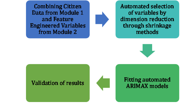
Figure 17. Flowchart of Module 3 analysis.
Data description
The input data for Module 3 of this project are
- Data for citizen geo-units from Module 1;
- Variables predicting the official stations as defined in Module 2;
- Satellite data on topography of Sofia to plot the results in
Data preparation
The first step of the data preparation at this phase is to create a single matrix with all features derived in Module 2 and described in section 4.2.4 above. This matrix would later serve as the exogenous factors to be plugged into the ARIMAX models for each geo-unit. Our assumption here is that if these features predict the PM10 from the official stations well, as proven in p.4.2.6 above, then these features would predict the citizen stations measurements as well. After taking into consideration the repeating variables, we bind the 5 datasets used for prediction of the official stations' measurements to create a matrix with 27 variables, aggregated on a daily base.
Next we take the data for the PM10 measurements for all 127 geo units as defined in Module 1. This data is also aggregated on a daily base, as is the matrix with 27 exogenous variables. We take the data for each of the geo units and add to them the exogenous variables for the respective day. These feature matrices that would be used for the predictive model building for each of the 127 geo units.
Preliminary Analysis
A main step in the preliminary analysis of the data in this module is analyzing common observations and selecting proper period to predict. The importance of this process derives from the fact that we need to have a single date to predict and compare the results from our modeling on one hand, and on the other – we need to be able to show predictions on the territory of Sofia for a specific day, instead of different points of time. The dataset with from Module 1 has ensured that all 127 geo units contain coherent and consistent data and here we're going to select a single date to train and test our models on.
The starting point of this analysis is to find the dates for which we have the most observations. A look at the data shows that the date with the most observations is 26th March 2018, when 112 of the 127 geo units have recorded PM10 concentration. Although the big amount of observations, we're going to skip that date and search for another one, since we know that the observations for the official stations, and respectively the matrix with exogenous variables we defined in p.5.2.2. have observations from December 2017 and the training period for our models would be too short.
The analysis shows that the next dates with the most observations recorded from different geo units are all dates between 08th May and 23rd June 2018 where 81 geo units contain data on PM10 concentration. As our goal is to have a dataset with as many observations as possible, we select the last date from this period, namely "2018-06-23". This is going to be the last date for the time series for all geo units and is going to be one of the dates for which we would later test our models.
Slicing the datasets on the 23rd of June decreases the number of geo units from 127 to 81. This is still a very good number of stations and that would be spread around the are Sofia area. We also checked whether there are no geo units with less than 30 days of observations, in order to have enough training data for the models as the assumption here is that if the geo unit has less than a month of observations, then it might not contain enough data to capture trends and seasonality. Luckily 81 all geo units have more than one month of observations.
After we now have the last date of our time series, additional checks are performed in order to ensure there is no missing values, i.e. we have full observations for each geo-unit. That manly concerns observations before 2018-01-01, since that's the date we have observations from for all 5 datasets from Module 2. The goal here is to exclude the option of additional interpolation and perform modeling based on the actual values we have for each geo unit.
Feature Engineering
In order to define the best possible set of predictors for each of our models in Module 3, we have used the so-called Lasso method. In statistics and machine learning, Lasso (least absolute shrinkage and selection operator; also Lasso or LASSO) is a regression-based method that performs variable selection in order to improve the the prediction accuracy and also easily interpret the statistical model it creates.
We use LASSO to follow a principled way to reduce the number of features in each of our models. Lasso involves a penalty factor that determines how many features are retained. The penalty factor is chosen using a cross-validation procedure to ensure that the model will generalize well to future data samples. The optimal value of the lambda coefficient is selected after cross validation. As a shrinkage method, by penalizing the parameters, we can choose a level of the beta coefficients which explain the response variable above a certain level. That would allow us to use a dataset with less variables for optimizing modeling purposes.
Important prerequisite for LASSO is scaling the feature matrix. That's why the process we follow is: for each geo-unit we regularize the non-categorical variables in the exogenous feature matrix by taking out the mean and dividing by the standard deviation and add the already existing categorical variables. The result is plugged in into the LASSO regression with optimized penalty factor for each geo unit.
So far we have similar information for each geo unit and in the following steps we will define different variables for each of them using automated algorithms. The first change will come exactly from the LASSO method application as we're going to define a threshold for the beta coefficients in the models, which will result in a different dataset for each of the different geo units.
The threshold for the beta coefficients in each of the 81 models is set to 0.1. This more conservative approach is selected for a number of reasons:
- Features with really low importance that would not enhance the results for the model are removed;
- As we have multiple models that we aim to automate, this procedure will select predictors for each one;
- Having more predictors in a model would not decrease model accuracy. In the worst case scenario, we would have predictors that do not bring additional value to the model and the only cost is that their usage in the modelling phase requires more computing power.
Additional check is performed in order to exclude models that are being predicted only by the intercept, which would mean they cannot be predicted by any of the features, but by another process. Figure 18 shows the number of selected features for each geo unit:
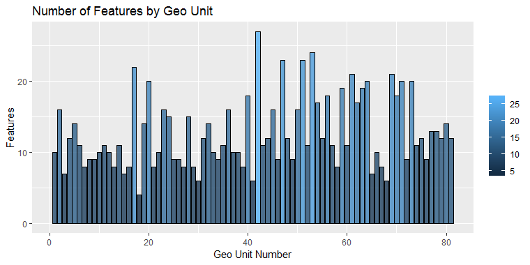
Figure 18: Number of selected features for each geo unit.
Apparently the algorithm has found different number of features for every geo unit. Table 8 provides summary of the details:
Table 8: Algorithm performance: summary details.
| Min. | 1st Qu. | Median | Mean | 3rd Qu. | Max. | |
|---|---|---|---|---|---|---|
| Number of features | 4.00 | 9.00 | 11.00 | 12.72 | 16.00 | 27.00 |
The minimum number of features that were selected after applying the LASSO method is 4. The average number of automatically selected features is between 12 and 13 and the algorithm has selected all of the 27 features for only one model. Figure 19 presents an example of the beta coefficients for geo-units 1 to 4. It is obvious that even for the first 4 geo units we have four different sets of predictors, each of them with different predicting power. For example, while Daily average relative humidity (RHAVG) might be the strongest positive predictor for geo units 1 and 4, geo unit 2's PM10 concentration is highly correlated to the levels of official station st9642 and geo unit 3's values are explained with the concentration of PM10 from official station 60881.
Based on this approach, we are able to automatically choose the best features that explain the response variable PM10 and we can start building each of the 81 models.
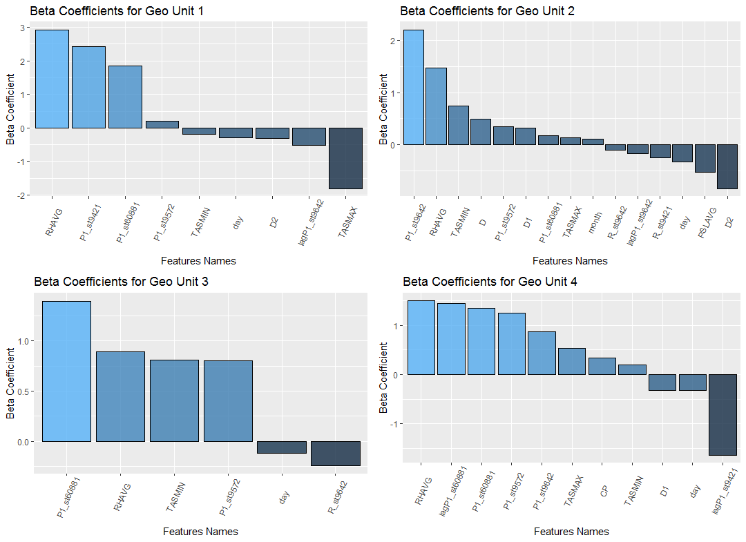
Figure 19:Example of the beta coefficients for geo-units 1 to 4.
Predictive modelling
The final number of stations explained in 5.2.3 results in the same number of models built as part of this research. Using different machine learning algorithms allowed us to automate the training process of each of these models and make them take into consideration the predictors and the fitting parameters valid for each model separately. In order to normalize and stabilize the variance of the PM10 particles, a logarithmic transformation is applied during the training process and then reverted to the original format for testing and validation purposes.
The predictive model used in this research is one of the most popular models for time series analysis and predictions – ARIMAX. ARIMAX is an acronym that stands for AutoRegressive Integrated Moving Average with Explanatory Variable. This model can be also considered as a multiple regression model with one or more autoregressive (AR) terms and one or more moving average (MA) terms.
ARIMAX models have all the standard fitting parameters as the ARIMA models. The p, d, q parameters in this research are defined by using out of the box function defined in R – auto.arima(). This function searches through combinations of order parameters and picks the set that optimizes the model fit criteria. After multiple loops and runs, it returns the best ARIMA model for each of the models according to either AIC, AICc or BIC value.
The explanatory variables adding the most value to the models are defined in 5.2.4. This part of the ARIMAX fitting process is also automated to be valid for each of the models separately meaning each model is trained with the best possible set of predictors.
Validation
There are plenty of options, indices and techniques which can be used to validate or verify the quality of the predictions. The most appropriate validation method should be selected after taking into consideration the specifics of the case study.
As explained in 5.2.3, due to the data availability, we had to choose the most appropriate day which will include as many observations and available stations as possible. Because of the low variability of observations in that day, we have decided to use the RMSE indicator as a main quality measure. Root Mean Square Error (RMSE) is basically the standard deviation of the residuals (prediction errors). It is a measure of how spread out these residuals are, or in other words, it demonstrates how concentrated the data is around the line of best fit.
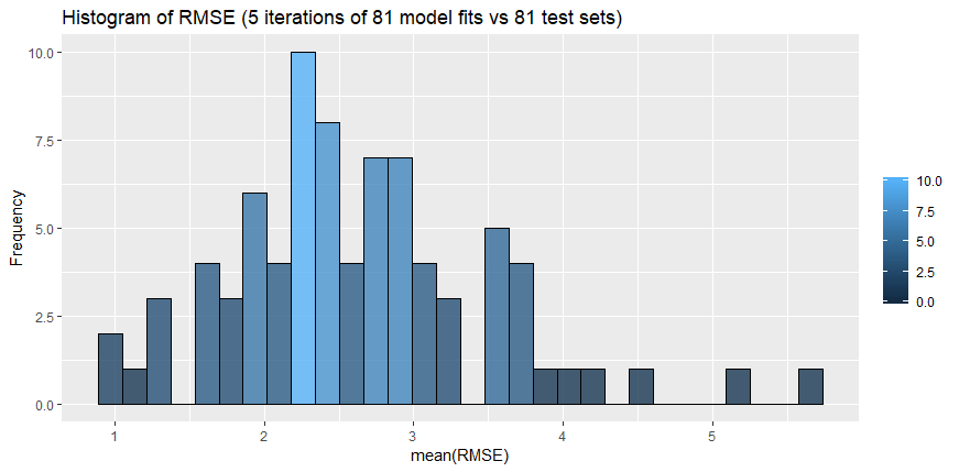
Figure 20: Histogram of RMSE.
Table 9 and Figure 20 are giving statistics of the RMSE value when comparing the prediction of the PM10 particles against the original PM10 values for that period for all the 81 stations and models available. For the purpose of the confirmation of the results and in order to avoid any random behavior, the model was built in an automated way which will allow it to run 5 times, taking 5 different periods to compare against.
Table 9: RMSE: summary information.
| Min. | 1st Qu. | Median | Mean | 3rd Qu. | Max. | |
|---|---|---|---|---|---|---|
| RMSE | 0.9923 | 2.0790 | 2.4402 | 2.6234 | 3.0528 | 5.6786 |
Code
Download the R code here… Download the data here…
Set up environment
rm(list=ls())
gc()
Set the path of the folder with data
setwd("/data")
Import data on EEU measurements for 2017 and 2018
eeu=list.files(path="/data",pattern="BG*")
ddeu=lapply(eeu,read.csv,na.string=c("","NA"," "), stringsAsFactors = F, fileEncoding="UTF-16LE")
Name data sets by stations
for (i in 1:length(eeu)){
  eeu[i]=gsub("BG_5_","st", eeu[i])
  eeu[i]=gsub("_timeseries.csv","", eeu[i])
  names(ddeu)[i]=eeu[i]
}
rm(eeu,i)
Select only the observations with averaging time == “hour”
for (i in 1:length(ddeu)){
  ddeu[[i]]=ddeu[[i]][ddeu[[i]]$AveragingTime=="hour",]
}

count = 0
i = 1
while(0 == 0){
  if (count == 1){
    i = i - 1
  }
  if(i > length(ddeu)){
    break
  }
  count = 0
  if(dim(ddeu[[i]])[1] == 0){
    ddeu[[i]] = NULL
    count = 1
  }
  i = i + 1
}
rm(count,i)
Check variables’ class of ddeu
sapply(lapply(ddeu,"[", ,"DatetimeEnd"),class)
sapply(lapply(ddeu,"[", ,"Concentration"),class)
Fix the class of the time variable
if(!require(lubridate)){
  install.packages("lubridate")
  library(lubridate)
}
for (i in 1:length(ddeu)){
  ddeu[[i]]=ddeu[[i]][,c("DatetimeEnd","Concentration")]
  ddeu[[i]]$DatetimeEnd=ymd_hms(ddeu[[i]]$DatetimeEnd, tz="Europe/Athens")
  colnames(ddeu[[i]])=c("time","P1eu")
}

sapply(lapply(ddeu,"[", ,"time"),class)
Make a time vecor with hourly sampling rate
teu=list()
for (i in 1:length(ddeu)){
  teu[[i]]=as.data.frame(seq.POSIXt(from=min(ddeu[[i]]$time),to=max(ddeu[[i]]$time), by="hour"))
  colnames(teu[[i]])[1]="time"
}
Make a list of time series on official P10 concentration for every station
if(!require(dplyr)){
  install.packages("dplyr")
  library(dplyr)
}

if(!require(devtools)){
  install.packages("devtools")
  library(devtools)
}

for (i in 1:length(ddeu)){
  teu[[i]]=left_join(teu[[i]],ddeu[[i]],by="time")
}
names(teu)=names(ddeu)
Bind datasets 2017 and 2018 for each of the official points
teu$st9421=bind_rows(teu$st9421_2017,teu$st9421_2018)
teu$st9572=bind_rows(teu$st9572_2017,teu$st9572_2018)
teu$st9616=bind_rows(teu$st9616_2017,teu$st9616_2018)
teu$st9642=bind_rows(teu$st9642_2017,teu$st9642_2018)
teu$st60881=teu$st60881_2018

teu=teu[c("st9421", "st9572","st9616","st9642","st60881")]
for (i in 1:length(teu)){
  colnames(teu[[i]])[2]="P1"}
rm(i,ddeu)
Check for duplicates
sapply(teu,dim)[1,]
sum(duplicated(teu[[1]]$time)) #0
sum(duplicated(teu[[2]]$time)) #0
sum(duplicated(teu[[3]]$time)) #0
sum(duplicated(teu[[4]]$time)) #0
sum(duplicated(teu[[5]]$time)) #0
Interpolate missing values for P1eu
if(!require(imputeTS)){
  install.packages("imputeTS")
  library(imputeTS)
}
Check the numer of missing obs
sapply(sapply(teu,is.na),sum)
sapply(sapply(teu,is.na),sum)/sapply(teu,dim)[1,]
Apply linear interpolation
for (i in 1:length(teu)){
  teu[[i]][,2]=na.interpolation(teu[[i]][,2], option="linear")
}
rm(i)
Aggregate official measuremnets on daily basis
Extract date from the time variable
for (i in 1:length(teu)){
  teu[[i]]$date=date(teu[[i]]$time)
}

names(aeu)=names(teu)
Import data on weather metrics
Import data on weather
setwd("C:\\Users\\O38648\\Box Sync\\R Scripts\\Projects\\AirPollutionFEBA\\data\\METEO-data")
ww=read.csv("lbsf_20120101-20180917_IP.csv",na.string=c("","NA"," ",-9999), stringsAsFactors = F)
Get a date vector
ww$date=make_date(year=ww$year,month=ww$Month,day=ww$day)
ww=ww[,c(23,1:22)]
Check for poorly populated variables
colSums(is.na(ww))
ww$date[is.na(ww$VISIB)==T]
Entire period for PRCPMAX and PRCPMIN is missing Last two months (Aug and Sep 2018) for VISIB are missing Remove this variables from the sample
ww=ww[,!names(ww) %in% c("PRCPMAX","PRCPMIN","VISIB","year","Month","day")]
Merge data on P10 and weather
for (i in 1:length(aeu)){
  aeu[[i]]=left_join(aeu[[i]],ww,by="date")
  aeu[[i]]$day=wday(aeu[[i]]$date,label=T)
}
Handle missing values
sapply(sapply(aeu,is.na),colSums)

for (i in 1:length(aeu)){
  aeu[[i]][,3:18]=sapply(aeu[[i]][,3:18],na.interpolation,option="linear")
}
rm(ww,i)
Look at the data first
Construct correlation matrix
cc=list()
for (i in 1:length(aeu)){
  cc[[i]]=cor(aeu[[i]][,2:18])
}
names(cc)=names(aeu)
Visualize correlation matrix
if(!require(plotly)){
  install.packages("plotly")
  require(plotly)
}
if(!require(RColorBrewer)){
  install.packages("RColorBrewer")
  require(RColorBrewer)
}
i=1 \# Change i=1,2,3,4,5 so as to get plot for each station
plot_ly(x=rownames(cc[[i]])[1:nrow(cc[[i]])], y=colnames(cc[[i]])[nrow(cc[[i]]):1],z=abs(cc[[i]][nrow(cc[[i]]):1,1:nrow(cc[[i]])]),type="heatmap",colors=brewer.pal(8,"Reds"))
Stationarity tests
if(!require(tseries)){
  install.packages("tseries")
  require(tseries)
}
aux=list()
for (i in 1:length(aeu)){
  a=adf.test(aeu[[i]]$P1)
  aux[[i]]=c(a$statistic,a$p.value)
  rm(a)
}
aux=as.data.frame(aux)
colnames(aux)=names(aeu)
rownames(aux)=c("ADF statistics", "p-value")
Feature engineering
eu=list()
for (i in 1:length(aeu)){
  eu[[i]]=aeu[[i]][,c("date","P1","TASMAX","TASMIN","RHAVG","PSLAVG","day")]
  eu[[i]]$lagP1=dplyr::lag(eu[[i]]$P1,1)
  eu[[i]]$month=month(aeu[[i]]$date)
  eu[[i]]$D1=ifelse(aeu[[i]]$RHMAX==100,1,0)
  eu[[i]]$D2=ifelse(aeu[[i]]$sfcWindMIN==0,1,0)
  eu[[i]]$D3=ifelse(aeu[[i]]$PRCPAVG==0,1,0)
  eu[[i]]$D=eu[[i]]$D1*eu[[i]]$D2*eu[[i]]$D3
  eu[[i]]$CP=aeu[[i]]$sfcWindAVG*(dplyr::lag(aeu[[i]]$sfcWindAVG,1))
  eu[[i]]$R=eu[[i]]$lagP1/eu[[i]]$CP
  eu[[i]]=eu[[i]][-1,]
}
names(eu)=names(aeu)

rm(aeu,aux,cc,teu,i)

for(i in 1:length(eu)){
  print(names(eu[[i]]))
}

for (i in 1:length(eu)){
  eu[[i]]<-eu[[i]][,c(1,3:7,9:14,2,8,15)]
  names(eu[[i]])[which(names(eu[[i]])=="P1")]<-paste0("P1_",names(eu)[i])
  names(eu[[i]])[which(names(eu[[i]])=="lagP1")]<-paste0("lagP1_",names(eu)[i])
  names(eu[[i]])[which(names(eu[[i]])=="R")]<-paste0("R_",names(eu)[i])
}
Create a data frame with all meteo features and the engineered features from module 2
meu<-eu[[1]]
if(!require(plyr)){
  install.packages("plyr")
  require(plyr)
}

for (i in 2:length(eu)){
  meu<-as_tibble(join_all(list(meu, eu[[i]][,c(1,13:15)]), by = "date"))
}
rm(eu)
setwd("/")
load("./citizenDaily.RData") \# Load output file from module 1 - a list of clusters
Selecting a date to train models
AllCitizenDaily <- do.call(bind_rows,citizenDaily)
summary(as.factor(AllCitizenDaily$date))[1:50]
The date with the most observations in the dataset “2018-03-26”. However, at this date we would only have less than three months of data for training the models.
The next date with the most observations in the dataset is “2018-06-23” - let’s use that as a reference
The analysis below is done twice with both dates
rm(AllCitizenDaily, i)

for (i in 1:length(citizenDaily)){
  citizenDaily[[i]]<-citizenDaily[[i]][which(citizenDaily[[i]]$date<="2018-06-23"),]
}


empty_clusters<-vector()
for (i in 1:length(citizenDaily)){
  if (length(rownames(citizenDaily[[i]]))<=30)
 {
    empty_clusters<-c(empty_clusters, i) # Mark clusters with no observations, or clusters which final date is before 2018-06-23
  }
}

if (length(empty_clusters)<=1){
  print("All clusters' have more than one observations before th selected date")
} else {
  citizenDaily<-citizenDaily[-empty_clusters]
}
As a result of this operation, we have clusters with observations until the selected date above
rm(empty_clusters, i)

empty_clusters<-vector()
for (i in 1:length(citizenDaily)){
  if (citizenDaily[[i]]$date[length(citizenDaily[[i]]$date)]!="2018-06-23")
  {
    empty_clusters<-c(empty_clusters, i) # Mark clusters with no observations, or clusters which final date is before 2018-06-23
  }
}

if (length(empty_clusters)<=1){
  print("All clusters' observations finish at the selected date date")
} else {
  citizenDaily<-citizenDaily[-empty_clusters]
}

rm(empty_clusters, i)
Additional columns for each cluster
for (i in 1:length(citizenDaily)){
  citizenDaily[[i]]<-as_tibble(join_all(list(citizenDaily[[i]], meu), type = "left", by = "date"))
}
rm(meu)
Handle missing values - this process ensures that all clusters have complete information about all variables
for (i in 1:length(citizenDaily)){
  citizenDaily[[i]] <- citizenDaily[[i]][complete.cases(citizenDaily[[i]]),]
}
Choose the optimal parameters for each cluster using Lasso regression
set.seed(123)

if (!require(glmnet)) {
  install.packages("glmnet")
  require(glmnet)
}
We’re going to use the Lasso regression to find the optimal features to predict the P1 for each cluster
Setting the threshold for the beta values
thresholdForBeta<-0.1
Creating a list with features for each cluster
feat<-list()
Changing the class of the factor variables and ordering the variables so that it is easier to perform the automatic feature selection in the next step
for (i in 1:length(citizenDaily)){
  citizenDaily[[i]]$day<-as.factor(citizenDaily[[i]]$day)
  citizenDaily[[i]]$month<-as.factor(citizenDaily[[i]]$month)
  citizenDaily[[i]]$D1<-as.factor(citizenDaily[[i]]$D1)
  citizenDaily[[i]]$D2<-as.factor(citizenDaily[[i]]$D2)
  citizenDaily[[i]]$D3<-as.factor(citizenDaily[[i]]$D3)
  citizenDaily[[i]]$D<-as.factor(citizenDaily[[i]]$D)
  citizenDaily[[i]]<-citizenDaily[[i]][,c(3, \# P1
                                          10:15, \# Factor variables: day, month, D1, D2, D3, D
                                          6:9, 16:31,  \# all remaining variables
                                          1:2, \# date, geohash
                                          4:5)] \# lng, lat

}
Applying the Lasso method with a dataframe scaled for the non-factor variables
citizenDaily_scaled<-list()
for (i in 1:length(citizenDaily)){
  citizenDaily_scaled[[i]]<-citizenDaily[[i]][,-(28:31)]
  citizenDaily_scaled[[i]][,2:7]<-citizenDaily_scaled[[i]][,2:7]
  citizenDaily_scaled[[i]][,8:27]<-scale(citizenDaily_scaled[[i]][,8:27], center = TRUE, scale = TRUE)
  eq1<-cv.glmnet(x=data.matrix(citizenDaily_scaled[[i]][,2:length(names(citizenDaily_scaled[[i]]))]),
                 y=as.numeric(citizenDaily_scaled[[i]]$P1),
                 alpha=1)
  eq2<-glmnet(x=data.matrix(citizenDaily_scaled[[i]][,2:length(names(citizenDaily_scaled[[i]]))]),
              y=as.numeric(citizenDaily_scaled[[i]]$P1),
              lambda=eq1$lambda.min)
  feat[[i]]=as.data.frame(eq2$beta[which(abs(eq2$beta)>thresholdForBeta),])
}

names(citizenDaily_scaled)<-names(citizenDaily)
names(feat)<-names(citizenDaily)
rm(eq1, eq2)
Change i=1…81 to see feature importance for each geo unit
i=1
{
  dd_importance<-feat[[i]]
  dd_importance<-dd_importance[order(dd_importance[,1], decreasing = T),, drop=FALSE]
  dd_importance$Features<-rownames(dd_importance)
  colnames(dd_importance)<-c("Beta","Features")
  dd_importance$Features <- factor(dd_importance$Features)

  title_name<-paste0("Beta Coefficients from LASSO Method for Geo Unit ",i)
  ggplot(data=dd_importance, aes(x=reorder(Features,-Beta), y=Beta)) +
    geom_bar(stat="identity",aes(fill=Beta), alpha = 0.8, col="black")+
    theme(axis.text.x = element_text(angle=65, vjust=0.6))+scale_x_discrete()+
    scale_fill_gradient("") +
    labs(title=title_name) +
    labs(x="Features Names", y ="Beta Coefficient from LASSO")
}
The feat list represents a list with the features that have the highest impact on the response variable P1 for each of the clusters
Now let’s create a list with dataframes containing the response variable and the features with the highest impact for each cluster
model_list<-list()
empty_models<-vector()
#save.image(file = "beforemodelling.RData")
#load("beforemodelling.RData")
for (i in 1:length(feat)){
  if (length(rownames(feat[[i]]))<=1) {
    empty_models<-c(empty_models, i) # Mark clusters for which no features were selected by Lasso except for the intercept
    model_list[[i]]<-citizenDaily[[i]][,c("date", "P1")]
  } else {
    model_list[[i]]<-citizenDaily[[i]][,c("date","geohash","lng","lat", "P1",c(rownames(feat[[i]])))]
    }
}

names(model_list)<-names(citizenDaily)
Remove clusters for which no features were selected by Lasso except for the intercept
if (length(empty_models)==0){
  model_list_final_full<-model_list
  print("There are no clusters with less than one beta coefficient")
} else {
  model_list_final_full<-model_list[-empty_models]
}

rm(model_list, empty_models) # Maybe remove citizenDaily, citizenDaily_scaled, feat, i, thresholdForBeta
Create a shorter dataframe for the modelling. Later we’ll get back to the geohash and coordinates
model_list_final_short<-list()

for (i in 1:length(model_list_final_full)){
  model_list_final_short[[i]]<- model_list_final_full[[i]][,-c(2:4)]
}

names(model_list_final_short)<-names(model_list_final_full)

if (!require(ggplot2)) {
  install.packages("ggplot2")
  require(ggplot2)
}
Number of Features by Geo Unit Barchart
dd_len<-vector()
for (i in 1:length(model_list_final_full)){
  dd_len<-c(dd_len,length(model_list_final_full[[i]][,5:length(colnames(model_list_final_full[[i]]))]))
}

dd_len<-as.data.frame(dd_len)
dd_len$geo_units<-seq(1,length(dd_len$dd_len), by=1)

summary(dd_len)
barplot(dd_len$dd_len)
hist(dd_len$dd_len, breaks = 30)
class(dd_len)

ggplot(data=dd_len, aes(x=geo_units, y=dd_len)) +
  geom_bar(stat="identity",aes(fill=dd_len), alpha = 0.8, col="black")+
  scale_fill_gradient("") +
  labs(title="Number of Features by Geo Unit") +
  labs(x="Geo Unit Number", y ="Features")
\# Exported as 760 * 380

summary(dd_len$dd_len)
Building prediction models
You can clean all the environment before modelling
save(cluster_list_ver3, file="cluster_list_ver3")
rm(list=ls())
load("cluster_list_ver3")
Step 1 Divide dataset into training and test set
rmse<-list()
for(k in 5:1){
First, let’s create two lists for training and test data
train_list<-list()
test_list<-list()

for (i in 1:length(model_list_final_short)){
  train_list[[i]]<-data.frame()
  test_list[[i]]<-data.frame()
}
names(train_list)<-names(model_list_final_short)
names(test_list)<-names(model_list_final_full)
rm(i)
For testing purposes, we would separate all values except for the last one !!! NB: Here we test five times the dataset vs each of the 5 last days
if (!require(lubridate)) {
  install.packages("lubridate")
  require(lubridate)
}

for (i in 1:length(model_list_final_short)){
  train_list[[i]]<-model_list_final_short[[i]][1:(length(rownames(model_list_final_short[[i]]))-(1+(k-1))),] # all observations except for the last one
  test_list[[i]]<-model_list_final_short[[i]][(length(rownames(model_list_final_short[[i]]))-(k-1)),] # the last observation
}
Step 2: Build the prediction model
if (!require(forecast)) {
  install.packages("forecast")
  require(forecast)
}

arima_list<-list()
Our prediction models for each geo unit would be based on the ARIMA-X model, which is an ARIMA model with external factors. The order of the ARIMA models is defined by the R’s built in auto.arima function. The external factors for each model are different, based on the feature selection procedure above. The result of this procedure would be a list of different model for each geo unit. NB: THIS LOOP TAKES SOME TIME TO RUN!!!
for (i in 1:length(train_list)){
  arima_list[[i]]<-arima(x = log(train_list[[i]]$P1), # ARIMA
                         order=arimaorder(auto.arima(train_list[[i]]$P1)), # ORDER - for each geo unit
                         xreg = data.matrix(train_list[[i]][,3:length(colnames(train_list[[i]]))])) # external variables
}


names(arima_list)<-names(train_list)
ACCURACY OF THE MODELS
results <- list()
for (i in 1:length(test_list)){

  results[[i]] <- predict(arima_list[[i]], newxreg = data.matrix(test_list[[i]][,3:length(colnames(test_list[[i]]))]))

}
Step 3: Check the accuracy of the model
RMSE
final <- list()
for (i in 1:length(arima_list)){
  final[[i]] <- data.frame(
    "P1" = model_list_final_full[[i]][length(rownames(model_list_final_full[[i]])),which(colnames(model_list_final_full[[1]])=="P1")],
    "P1_Predicted" = exp(as.numeric(results[[i]])[1]),
    "RMSE" = accuracy(f=exp(as.numeric(results[[i]])[1]),x=as.numeric(test_list[[i]]$P1))[2], #accuracy(arima_list[[i]])[2],
    "lng" = model_list_final_full[[i]][1,which(colnames(model_list_final_full[[1]])=="lng")],
    "lat" = model_list_final_full[[i]][1,which(colnames(model_list_final_full[[1]])=="lat")])
  }

names(final)<-names(model_list_final_full)
dd <- as.data.frame(matrix(unlist(final),nrow=length(final), byrow=T))
colnames(dd)<-colnames(final[[1]])

rmse[[k]]<-dd$RMSE
}
get the mean of the RMSE value of the 5 runs for each geounit
rmse <- as.data.frame(matrix(unlist(rmse), nrow=length(unlist(rmse[1]))))
rmse$RMSE_MEAN <- rowMeans(rmse)
summary(rmse$RMSE_MEAN)
plot a histgoram of the RMSE’s mean
ggplot(data=rmse, aes(rmse$RMSE_MEAN)) +
  geom_histogram(col="black",
                 aes(fill=..count..),
                 alpha = 0.8) +
  scale_fill_gradient("") +
  labs(title="Histogram of RMSE (5 iterations of 81 model fits vs 81 test sets)") +
  labs(x="mean(RMSE)", y="Frequency")

dd_map<-dd[,c(which(colnames(dd)==c("lng")),which(colnames(dd)==c("lat")))]

if (!require(leaflet)) {
  install.packages("leaflet")
  require(leaflet)
}

dd_map %>%
  leaflet() %>%
  addTiles() %>%
  addCircleMarkers(weight = 3, color = "blue")
Step 4: Prepare for Shiny build a dataset to feed the shiny app - https://sofiaairfeba.shinyapps.io/feba_sofia_air/ 3 types of observations for PM10 are needed - yesterday’s, today’s and the predicted one for tomorrow
shiny_set <- list()
for (i in 1:length(arima_list)){

  shiny_set[[i]] <- data.frame(
    "geohash" = model_list_final_full[[i]][1,which(colnames(model_list_final_full[[1]])=="geohash")],
    "lat" = model_list_final_full[[i]][1,which(colnames(model_list_final_full[[1]])=="lat")],
    "lng" = model_list_final_full[[i]][1,which(colnames(model_list_final_full[[1]])=="lng")],
    "P1" = model_list_final_full[[i]][length(rownames(model_list_final_full[[i]]))-2,which(colnames(model_list_final_full[[1]])=="P1")],
    "P1.1" = model_list_final_full[[i]][length(rownames(model_list_final_full[[i]]))-1,which(colnames(model_list_final_full[[1]])=="P1")],
    "P1.2" = exp(as.numeric(results[[i]])[1]))
}
export .csv to feed the Shiny app
write.csv(ldply(shiny_set, data.frame), file = "/sofia_summary.csv", row.names = FALSE, na = "")
[Acknowledgment] [Introduction] [Methodology] [Bias correction] [Analysis] [Features] [Prediction] [Summary]