Data Analysis (Module 2, p. 2/2)

Appendix Module 2

Full correlation matrix (by all stations) here…

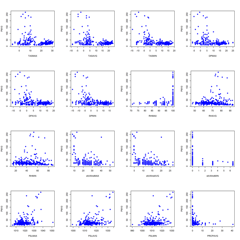
Pairwise scatterplots for station 9572
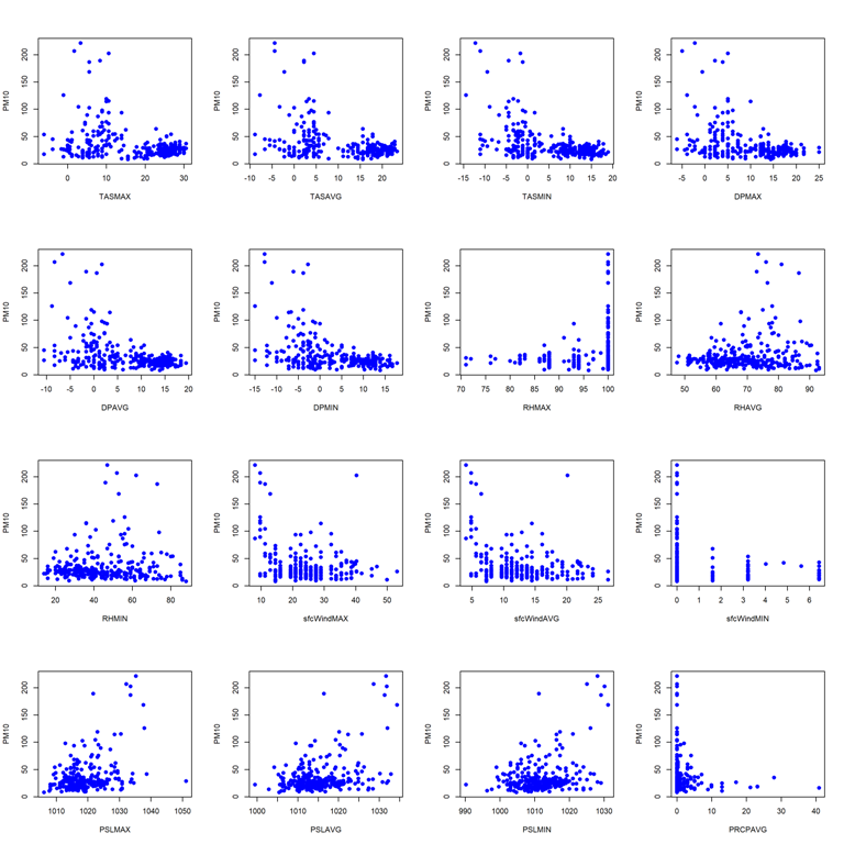
Pairwise scatterplots for station 9616
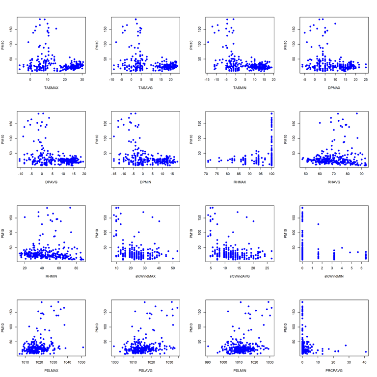
Pairwise scatterplots for station 9642
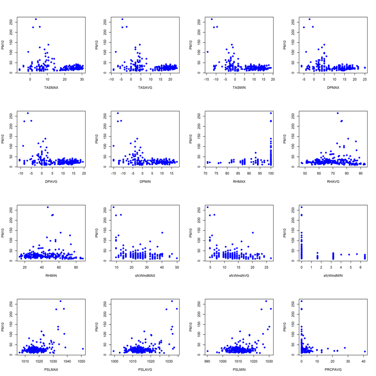
Pairwise scatterplots for station 60881

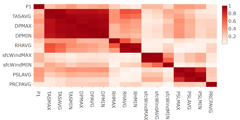
Plot of the correlation matrix in absolute terms for station 9572
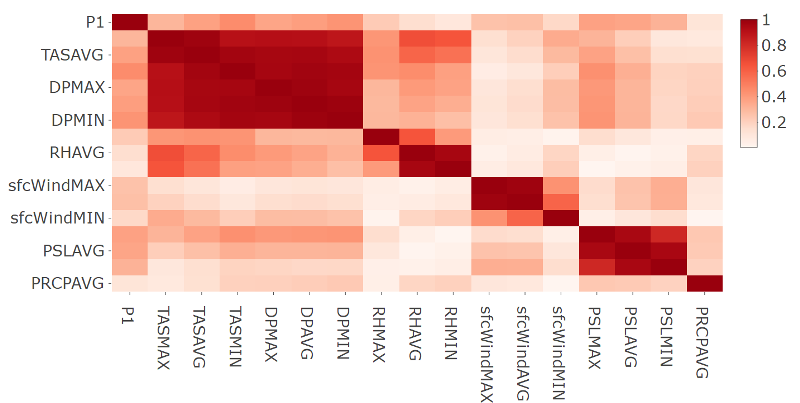
Plot of the correlation matrix in absolute terms for station 9616
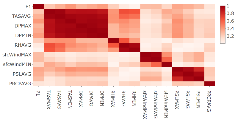
Plot of the correlation matrix in absolute terms for station 9642
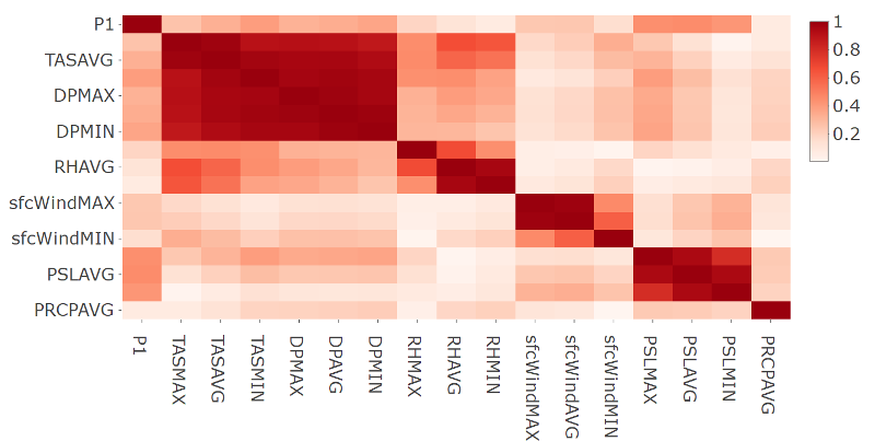
Plot of the correlation matrix in absolute terms for station 60881

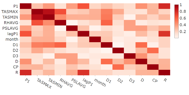
Plot of the correlation matrix in absolute terms for the response and selected features variables for station 9572
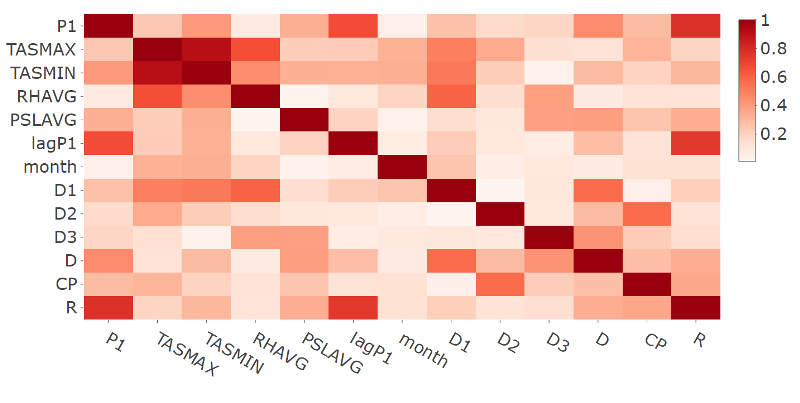
Plot of the correlation matrix in absolute terms for the response and selected features variables for station 9616
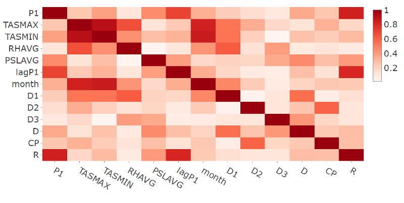
Plot of the correlation matrix in absolute terms for the response and selected features variables for station 9642
Plot of the correlation matrix in absolute terms for the response and selected features variables for station 60881

Plot: Summary of feature importance expressed as percentage of the cumulative decrease in the optimized loss function. Station 9572
Plot: Summary of feature importance expressed as percentage of the cumulative decrease in the optimized loss function. Station 9616
Plot: Summary of feature importance expressed as percentage of the cumulative decrease in the optimized loss function. Station 9642
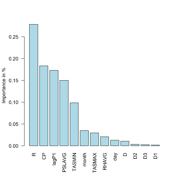
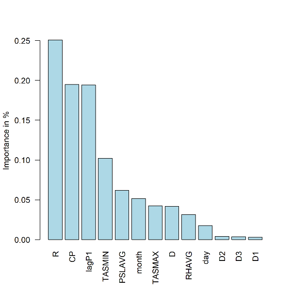
Plot: Summary of feature importance expressed as percentage of the cumulative decrease in the optimized loss function. Station 60881

Code

Download the R code here… Download the data here…

Set up environment

rm(list=ls())
gc()

Set the path of the folder with data

setwd("/data")

Import data on EEU measurements for 2017 and 2018

eeu=list.files(path="/data",pattern="BG*")
ddeu=lapply(eeu,read.csv,na.string=c("","NA"," "), stringsAsFactors = F, fileEncoding="UTF-16LE")

Name data sets by stations

for (i in 1:length(eeu)){
  eeu[i]=gsub("BG_5_","st", eeu[i])
  eeu[i]=gsub("_timeseries.csv","", eeu[i])
  names(ddeu)[i]=eeu[i]
}
rm(eeu,i)

Select only the observations with averaging time == “hour”

for (i in 1:length(ddeu)){
  ddeu[[i]]=ddeu[[i]][ddeu[[i]]$AveragingTime=="hour",]
}

count = 0
i = 1
while(0 == 0){
  if (count == 1){
    i = i - 1
  }
  if(i > length(ddeu)){
    break
  }
  count = 0
  if(dim(ddeu[[i]])[1] == 0){
    ddeu[[i]] = NULL
    count = 1
  } 
  i = i + 1
}
rm(count,i)

Check variables’ class of ddeu

sapply(lapply(ddeu,"[", ,"DatetimeEnd"),class)
sapply(lapply(ddeu,"[", ,"Concentration"),class)

Fix the class of the time variable

if(!require(lubridate)){
  install.packages("lubridate")
  library(lubridate)
}
for (i in 1:length(ddeu)){
  ddeu[[i]]=ddeu[[i]][,c("DatetimeEnd","Concentration")]
  ddeu[[i]]$DatetimeEnd=ymd_hms(ddeu[[i]]$DatetimeEnd, tz="Europe/Athens")
  colnames(ddeu[[i]])=c("time","P1eu")
}

sapply(lapply(ddeu,"[", ,"time"),class)

Make a time vecor with hourly sampling rate

teu=list()
for (i in 1:length(ddeu)){
  teu[[i]]=as.data.frame(seq.POSIXt(from=min(ddeu[[i]]$time),to=max(ddeu[[i]]$time), by="hour"))
  colnames(teu[[i]])[1]="time"
}

Make a list of time series on official P10 concentration for every station

if(!require(dplyr)){
  install.packages("dplyr")
  library(dplyr)
}

if(!require(devtools)){
  install.packages("devtools")
  library(devtools)
}

for (i in 1:length(ddeu)){
  teu[[i]]=left_join(teu[[i]],ddeu[[i]],by="time")
}
names(teu)=names(ddeu)

Bind datasets 2017 and 2018 for each of the official points

teu$st9421=bind_rows(teu$st9421_2017,teu$st9421_2018)
teu$st9572=bind_rows(teu$st9572_2017,teu$st9572_2018)
teu$st9616=bind_rows(teu$st9616_2017,teu$st9616_2018)
teu$st9642=bind_rows(teu$st9642_2017,teu$st9642_2018)
teu$st60881=teu$st60881_2018

teu=teu[c("st9421", "st9572","st9616","st9642","st60881")]
for (i in 1:length(teu)){
  colnames(teu[[i]])[2]="P1"}
rm(i,ddeu)

Check for duplicates

sapply(teu,dim)[1,]
sum(duplicated(teu[[1]]$time)) #0
sum(duplicated(teu[[2]]$time)) #0
sum(duplicated(teu[[3]]$time)) #0
sum(duplicated(teu[[4]]$time)) #0
sum(duplicated(teu[[5]]$time)) #0

Interpolate missing values for P1eu

if(!require(imputeTS)){
  install.packages("imputeTS")
  library(imputeTS)
}

Check the numer of missing obs

sapply(sapply(teu,is.na),sum)
sapply(sapply(teu,is.na),sum)/sapply(teu,dim)[1,]

Apply linear interpolation

for (i in 1:length(teu)){
  teu[[i]][,2]=na.interpolation(teu[[i]][,2], option="linear")
}
rm(i)

Aggregate official measuremnets on daily basis

Extract date from the time variable

for (i in 1:length(teu)){
  teu[[i]]$date=date(teu[[i]]$time)
}

Aggregate data on daily basis

aeu=list()
for (i in 1:length(teu)){
  aeu[[i]]=teu[[i]] %>%
    group_by(date) %>%
    summarise(P1=mean(P1))
}
names(aeu)=names(teu)
#rm(teu,i)

Import data on weather metrics

Import data on weather

setwd("/")
ww=read.csv("lbsf_20120101-20180917_IP.csv",na.string=c("","NA"," ",-9999), stringsAsFactors = F)

Get a date vector

ww$date=make_date(year=ww$year,month=ww$Month,day=ww$day)
ww=ww[,c(23,1:22)]

Check for poorly populated variables

colSums(is.na(ww))
ww$date[is.na(ww$VISIB)==T]

Entire period for PRCPMAX and PRCPMIN is missing Last two months (Aug and Sep 2018) for VISIB are missing Remove this variables from the sample

ww=ww[,!names(ww) %in% c("PRCPMAX","PRCPMIN","VISIB","year","Month","day")]

Merge data on P10 and weather

for (i in 1:length(aeu)){
  aeu[[i]]=left_join(aeu[[i]],ww,by="date")
  aeu[[i]]$day=wday(aeu[[i]]$date,label=T)
}

Handle missing values

sapply(sapply(aeu,is.na),colSums)

for (i in 1:length(aeu)){
  aeu[[i]][,3:18]=sapply(aeu[[i]][,3:18],na.interpolation,option="linear")
}
rm(ww,i)

Look at the data first

Construct correlation matrix

cc=list()
for (i in 1:length(aeu)){
  cc[[i]]=cor(aeu[[i]][,2:18])
}
names(cc)=names(aeu)

Visualize correlation matrix

if(!require(plotly)){
  install.packages("plotly")
  library(plotly)
}
if(!require(RColorBrewer)){
  install.packages("RColorBrewer")
  library(RColorBrewer)
}
i=1 

Change i=1,2,3,4,5 so as to get plot for each station

plot_ly(x=rownames(cc[[i]])[1:nrow(cc[[i]])], y=colnames(cc[[i]])[nrow(cc[[i]]):1],z=abs(cc[[i]][nrow(cc[[i]]):1,1:nrow(cc[[i]])]),type="heatmap",colors=brewer.pal(8,"Reds"))

Stationarity tests

if(!require(tseries)){
  install.packages("tseries")
  library(tseries)
}
aux=list()
for (i in 1:length(aeu)){
  a=adf.test(aeu[[i]]$P1)
  aux[[i]]=c(a$statistic,a$p.value)
  rm(a)
}
aux=as.data.frame(aux)
colnames(aux)=names(aeu)
rownames(aux)=c("ADF statistics", "p-value")

Feature engineering

eu=list()
for (i in 1:length(aeu)){
  eu[[i]]=aeu[[i]][,c("P1","TASMAX","TASMIN","RHAVG","PSLAVG","day")]
  eu[[i]]$lagP1=dplyr::lag(eu[[i]]$P1,1)
  eu[[i]]$month=month(aeu[[i]]$date)
  eu[[i]]$D1=ifelse(aeu[[i]]$RHMAX==100,1,0)
  eu[[i]]$D2=ifelse(aeu[[i]]$sfcWindMIN==0,1,0)
  eu[[i]]$D3=ifelse(aeu[[i]]$PRCPAVG==0,1,0)
  eu[[i]]$D=eu[[i]]$D1*eu[[i]]$D2*eu[[i]]$D3
  eu[[i]]$CP=aeu[[i]]$sfcWindAVG*(dplyr::lag(aeu[[i]]$sfcWindAVG,1))
  eu[[i]]$R=eu[[i]]$lagP1/eu[[i]]$CP
  eu[[i]]=eu[[i]][-1,]
}
names(eu)=names(aeu)

Construct correlation matrix

cc=list()
for (i in 1:length(eu)){
  cc[[i]]=cor(eu[[i]][,!names(eu[[i]]) %in% "day"])
}
names(cc)=names(eu)

Visualize correlation matrix

i=1 ``` ```R Change i=1,2,3,4,5 so as to get plot for each station
plot_ly(x=rownames(cc[[i]])[1:nrow(cc[[i]])], y=colnames(cc[[i]])[nrow(cc[[i]]):1],z=abs(cc[[i]][nrow(cc[[i]]):1,1:nrow(cc[[i]])]),type="heatmap",colors=brewer.pal(8,"Reds"))

Random forest

mean absolute percentage error

MAE=list() 

root mean squared error

RMSE=list()

feature importance

FI=list() 
for (i in 1:length(eu)){
  FI[[i]]=data.frame(matrix(NA,ncol=1,nrow=13))
  FI[[i]][,1]=as.character(names(eu[[i]])[-1])
  colnames(FI[[i]])="fname"
}
names(FI)=names(eu)

for (t in 1:100){

Split data into training and test set

set.seed(t)
  
  train=list()
  for (i in 1:length(eu)){
    train[[i]]=sample(nrow(eu[[i]]),round(nrow(eu[[i]])/2))
  }

Model estimation & feature importance

if(!require(randomForest)){
    install.packages("randomForest")
    library(randomForest)
  }
  eq=list()
  for (i in 1:length(eu)){
    eq[[i]]=randomForest(P1~.,data=eu[[i]][train[[i]],])
    a=data.frame(fname=as.character(rownames(eq[[i]]$importance)), imp=as.numeric(eq[[i]]$importance))
    colnames(a)[2]=paste("imp",t,sep="")
    FI[[i]]=left_join(FI[[i]],a,by="fname")
    rm(mae,rmse,a)
  }

Calculate out-of-sample accuracy

  mae=data.frame(matrix(NA,nrow=length(eu),ncol=3))
  rownames(mae)=names(eu)
  colnames(mae)=c("M1","M2","M3")
  rmse=data.frame(matrix(NA,nrow=length(eu),ncol=3))
  rownames(rmse)=names(eu)
  colnames(rmse)=c("M1","M2","M3")
  
  for (i in 1:length(eu)){
    f=predict(eq[[i]],newdata=eu[[i]][-train[[i]],])
    rmse[i,"M1"]=sqrt(mean((eu[[i]]$P1[-train[[i]]]-mean(eu[[i]]$P1[-train[[i]]]))^2))
    rmse[i,"M2"]=sqrt(mean((eu[[i]]$P1[-train[[i]]]-eu[[i]]$lagP1[-train[[i]]])^2))
    rmse[i,"M3"]=sqrt(mean((eu[[i]]$P1[-train[[i]]]-f)^2))
    mae[i,"M1"]=mean(abs((eu[[i]]$P1[-train[[i]]]-mean(eu[[i]]$P1[-train[[i]]]))/eu[[i]]$P1[-train[[i]]]))
    mae[i,"M2"]=mean(abs((eu[[i]]$P1[-train[[i]]]-eu[[i]]$lagP1[-train[[i]]])/eu[[i]]$P1[-train[[i]]]))
    mae[i,"M3"]=mean(abs((eu[[i]]$P1[-train[[i]]]-f)/eu[[i]]$P1[-train[[i]]]))
  }
  MAE[[t]]=mae
  RMSE[[t]]=rmse
}

rm(i,t)

MAE=as.data.frame(MAE)
RMSE=as.data.frame(RMSE)

mae=data.frame(matrix(NA,nrow=length(eu),ncol=3))
rownames(mae)=names(eu)
colnames(mae)=c("M1","M2","M3")
rmse=data.frame(matrix(NA,nrow=length(eu),ncol=3))
rownames(rmse)=names(eu)
colnames(rmse)=c("M1","M2","M3")

Devrie rmse and mae

for (i in 1:length(eu)){
  mae[i,"M1"]=mean(as.numeric(MAE[i,grep("^M1",names(MAE))]))
  mae[i,"M2"]=mean(as.numeric(MAE[i,grep("^M2",names(MAE))]))
  mae[i,"M3"]=mean(as.numeric(MAE[i,grep("^M3",names(MAE))]))
  rmse[i,"M1"]=mean(as.numeric(RMSE[i,grep("^M1",names(RMSE))]))
  rmse[i,"M2"]=mean(as.numeric(RMSE[i,grep("^M2",names(RMSE))]))
  rmse[i,"M3"]=mean(as.numeric(RMSE[i,grep("^M3",names(RMSE))]))
}

Derive importance

fi=list()
for (i in 1:length(FI)){
  fi[[i]]=data.frame(fname=FI[[i]]$fname)
  fi[[i]]$fimp=apply(FI[[i]][,2:101],1,mean)
  fi[[i]]$pfimp=fi[[i]]$fimp/sum(fi[[i]]$fimp)
  rownames(fi[[i]])=FI[[i]]$fname
}

i=5 